RTG #1: Song lyrics
In this article, I’ll discuss a bit about my experience working with the 5 Million Song Lyrics Dataset, which contains data from Genius, a place where anyone can update information on songs from their favorite artists!
Loading the data
Unzipped, the dataset is almost 9GB in size, which makes it difficult to work with, especially when most of the size comes from big strings of text (the song lyrics) that are not efficiently stored. Under normal circumstances (16GB of RAM) we may manage to load it in memory, but operations that require creating a copy of the data will fail. This made preprocessing quite a pain.
To deal with that I decided to work with a toy dataset with 500,000 samples in the beginning, and when the time came to deal with the whole dataset, I would do that in batches. The situation was dire but it could be worse. I couldn’t process it in memory but at least I could load it, so the workflow of processing data in batches -> save to disk -> aggregate results and load to memory was still viable.
Pandas was the tool of choice for manipulating the data, mostly because of familiarity. Dask seemed like a great idea, but the formatting of the song lyrics made it not that useful (I’ll elaborate in the following section). After everything was mostly done, I came around Polars, which looked like a great candidate that I didn’t know existed.
What are we dealing with?
Normally songs are not formatted the same way normal text is, they are formatted much like poems, with a lot of line breaks and whitespaces. Our data captured this format literally with a lot of \n characters in the middle of the lyrics.
| Some samples of songs in this dataset |
|---|
| [Chorus: Opera Steve & Cam'ron]\nKilla Cam, Killa Cam, Cam\nKilla Cam, Killa… |
| [Produced by Irv Gotti]\n\n[Intro]\nYeah, hah, yeah, Roc-A-Fella\nWe invite you to… |
| Maybe cause I'm eatin\nAnd these bastards fiend for they grub\nI carry pumps… |
Those \n made Dask a poor choice. The whole idea of the library is to partition a DataFrame and process those partitions in parallel. Parallelism would be a great help here to clean the \ns from the lyrics, but the problem is that Dask counts newline characters as a way to create partitions, and having line endings in the lyrics messes everything up. To use Dask I would need to first remove all the \ns, but at this point, I could use the tool I used to remove them to do the whole processing.
Another thing you’ll notice about the lyrics is the presence of some indicators in square brackets, like [Chorus], [Intro], etc. This is Genius specific. If you browse any song on their website, odds are you’ll find something similar. They may convey some information about the lyrical structure, but as they can contain basically anything and not all songs have them, I decided to remove them.
The language barrier
Although I wasn’t aware at first, the dataset contained lyrics in many languages. My idea was to work with English only, so a way to identify the language of a song was needed.
Of course, this couldn’t be done manually for 5 million + songs, so I searched for some language identification methods and encountered CLD3, which worked ok but appeared inconsistent in my tests. Slight changes to the input often made a big difference in the predicted language.
1
2
3
4
5
6
7
8
9
>>> text = "I am at the Pizza Hut"
>>> gcld3_model.FindLanguage(text=text).language
'ca' # Catalan
>>> text = "I'mm at the Pizza Hut"
>>> gcld3_model.FindLanguage(text=text).language
'en' # English
>>> text = "I'm at the Pizza Hut"
>>> gcld3_model.FindLanguage(text=text).language
'mt' # Maltese
Then I encountered FastText, which among other things, does language identification. It appeared to be more consistent than CLD3, but wasn’t able to identify as many languages. In the end, I decided to combine their results, only labeling songs when both of the models agreed.
The language tag barrier
Combining the results of the two models was pretty easy on paper. If they both said a song was written in Filipino, the language was marked as “Filipino”. However, they don’t say “Filipino” the same way. They return a language tag, something like en, fr, pt, and the problem is that they don’t use the same set of tags. So while for CLD3, Filipino is fil, for FastText it is tl.
This was a big problem until I found langcodes, a library that was designed to deal with this kind of situation. It allowed me to retrieve the language name from the language tag, and then convert the name so that both models used the same tags for the same languages.
With that, I was able to work with songs that were written in English (most of the time). Multi-language NLP is something I’m not quite ready for yet. I also created a new Kaggle dataset with the language labels added. You can find it here.
Document representation
With the data we have to work with, I planned on running a clustering method to see if it was possible to create groups of songs based on the characteristics of their lyrics alone. The ideal scenario in this setting would be a model that could separate songs by genre by learning the specifics of songwriting for each genre. In order to do that, I needed a way to represent the songs in a machine-friendly format.
One way of doing that is using the classic TF-idf. This is a well-known technique that represents documents (in our case lyrics) using information like the frequency of words in the document and the number of documents that word appears in. The idea is that a document is considered more unique if a few sets of words occur many times in that document, but not many times in most of the other documents.
This time I tried a different approach. Instead of TF-idf, opted for something like word2vec. This technique consists of representing a word (a thing that most machine learning algorithms can’t operate with) as a vector (a thing that most machine learning algorithms can operate with). The tool of choice to achieve that was SpaCy, an NLP tool that seemed to do (more than) what I wanted effortlessly.
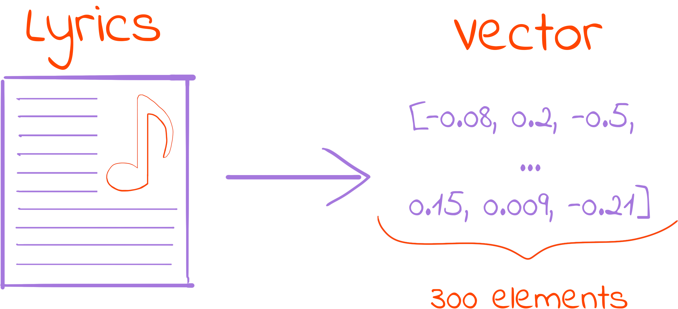
To do document representation as a vector, SpaCy uses a clever technique that first represents elements in the document as 300-dimensional vectors and then averages those vectors to represent the entire document. To make this possible in a reasonable amount of time, you can download models that contain the vector form for hundreds of thousands of constructs you may find in text, like words, punctuation symbols, whitespaces, etc.
We are now ready to cluster
Nothing fancy here. My strategy was just the plain old KMeans. I didn’t do any sort of analysis to define the optimal number of clusters because I had a clear goal in mind: We were working with 6 genres (rap, rb, rock, pop, misc, and country), so I went straight for 6 clusters. The results were not that great (euphemism).
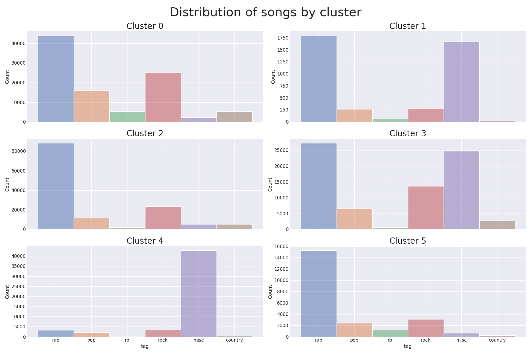
The figure above contains the song distribution by genre by cluster. In the ideal world, each cluster would contain only songs of a specific genre. In the picture, it would translate to 6 histograms, each of them with a single bar and each bar with a different color. This didn’t happen. Sadly.
Working with the full dataset
Everything went well with the toy dataset, but working with the full dataset made this one of the experiences of all time. I planned to do it all in a Kaggle notebook, as it has more RAM than my local machine and after searching for a bunch of ways to make the notebook use less memory, I was finally able to finish.
You can check the end result here. I still had to download cached results instead of doing everything from scratch as Kaggle notebook sessions last 12 hours max. Steps like generating the document representation or identifying the language of each song took multiple hours.
Conclusion
Songs are more than the lyrics alone, and the fact that I removed the song structure in the pre-processing step probably didn’t help in the clustering process. All in all the chance of creating a clustering method that learned song genres was pretty slim, but nonetheless, it was a cool experience. I would probably need to incorporate audio features into the data in order to have a better chance of succeeding.
Although I missed the main goal, I could at least derive some insight from this experience:
- The misc genre in Genius is mostly used to identify pieces that aren’t songs. This may seem obvious if you know Genius well, but I had no idea it contained poems, books, or even episode transcriptions. One of the clusters was somehow good at capturing the misc-labeled songs, so I decided to investigate.
- Genius started as Rap Genius, with a focus on hip-hop music. The rap genre had significant representation in the entire dataset and was the most popular genre in the sample I chose to work on.
For the next time, I think I’ll try to go with something that I can work on my local machine without much issue.