RTG #3: EDA on Yu-Gi-Oh!

This time we’ll use the Yu-Gi-Oh! Cards dataset to derive some insight on one of the most popular trading card games of all time.
The setting
Yu-Gi-Oh is my favorite card game. In fact, this website is named after one of its cards:
 Pacifis, the Phantasm City
This card is obnoxiously annoying, but I digress. Today’s RTG aims to answer some questions about how the game has evolved throughout the years using information on the entire Yu-Gi-Oh collection from YGOProDeck.
In the spirit of the RTG series, this post will talk about the decisions made, problems encountered, and lessons learned. The “real” analysis can be found in the Kaggle notebook or in the Github repository.
The data
YGOProDeck has a free API that allows anyone to query their entire card database. My original idea was to create a Kaggle dataset with that information. After a little bit of research, I found out that someone already did that in the form of the Yu-Gi-Oh! Cards dataset.
The only challenge in this part was how to correctly merge the available pieces of data. The execution was simple but required knowing a little about how Yu-Gi-Oh (YGO from now onwards) card releases work. Some things to keep in mind were:
- The same card can appear in multiple sets, in the form of a reprint
- Some cards have alternative artworks.Those cards do the exact same thing as the originals but are technically different because they use a different picture
Having done that, the data was ready for analysis. Some of the attributes available were:
| attribute | description |
|---|---|
| id | Card id. Not unique, as the same card can appear in another set |
| set_name | Name of the set in which this particular card appeared in |
| name | Name as its written on the card |
| desc | Card effect or description (big text) |
| type | If the card is a monster/spell/trap |
| attribute | Only available to monster cards. One of: EARTH, DARK, LIGHT, WATER, FIRE, WIND, DIVINE |
| upvotes | Number of upvotes in the YGOProDeck page |
The analysis
The first step was electing questions that could be answered with the information given:
- Which attribute has the most amount of supporting cards?
- What are some of the most loved/hated cards?
- When did special summoning start gaining popularity?
- Are we getting more or less reprints?
You can check my answer to those questions in the Kaggle notebook (or on github). Out of those, the most “technical” was question number 1. I’ll discuss my approach in the following section.
Attribute analysis
The initial question can be answered by calculating the frequency of each attribute (value_counts) without considering reprints and alternative artworks. However, to gain a more insightful view of the problem I decided to check how the distribution of attributes evolved as years passed.

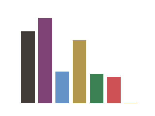 Number of cards by attribute
In order to do that, I needed a way to manipulate the date information. The original data used the following date format: YYYY-MM-DD. Converting it to the more desirable pd.datetime was quite simple, using the format attribute of Pandas’ to_datetime function.
1
2
3
df["date"] = pd.to_datetime(
    df["date"], format="%Y-%m-%d"
)
The second step was to group the data by year. groupby seemed to be the tool for the job. One interesting behavior of this function is that it can also group the data based on an arbitrary list or series, not only a column.
This means that we can create a series using only the year values from the dataset without adding it as a column on the dataframe. To create this series, the dt acessor object is our friend. With it, you can check information like the year, day, hour, and even time zones of an entire pd.datetime series.
1
grouped = df.groupby(df["date"].dt.year)["attribute"]
Now the tricky part is how to get this information in a usable format. The piece of code above created a bunch of groups (one group for each year), and each group has only a single column, the “attribute” column.
The most common step after a groupby operation is aggregation. The most common aggregations are something like computing averages, min or max values, counting values, etc. In this case, we’re interested in knowing the number of occurrences of each attribute in a given group (year). To achieve that we use the value_counts aggregation, something that was introduced in Pandas 1.4.
1
2
3
4
attr_by_year = (
    df.groupby(df["date"].dt.year)["attribute"]
    .value_counts()
)
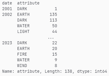
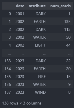
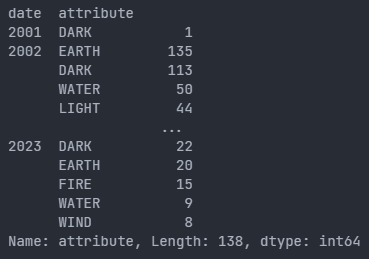 Getting the yearly frequency of each attribute
This ultimately did exactly what I wanted. However, the result of the aggregation is a multi-indexed series, which is hard to work with. The final step is converting it to a dataframe by turning the multi-index into multiple columns.
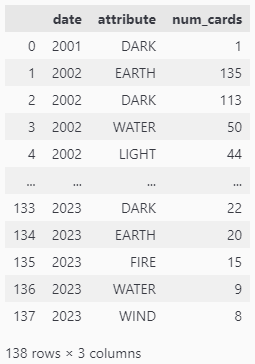
 Turning a multi-index into columns
Now the final step is to create a visualization. I opted for a stacked bar chart because it not only displays information about each attribute but also about all of them combined, giving a nice yearly overview.
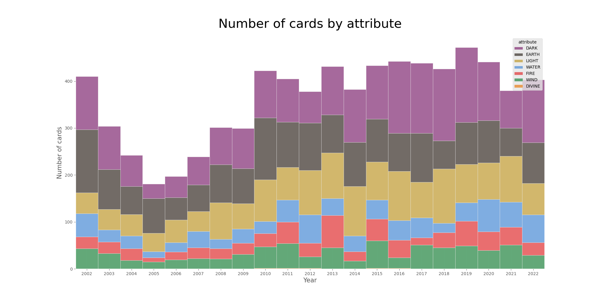
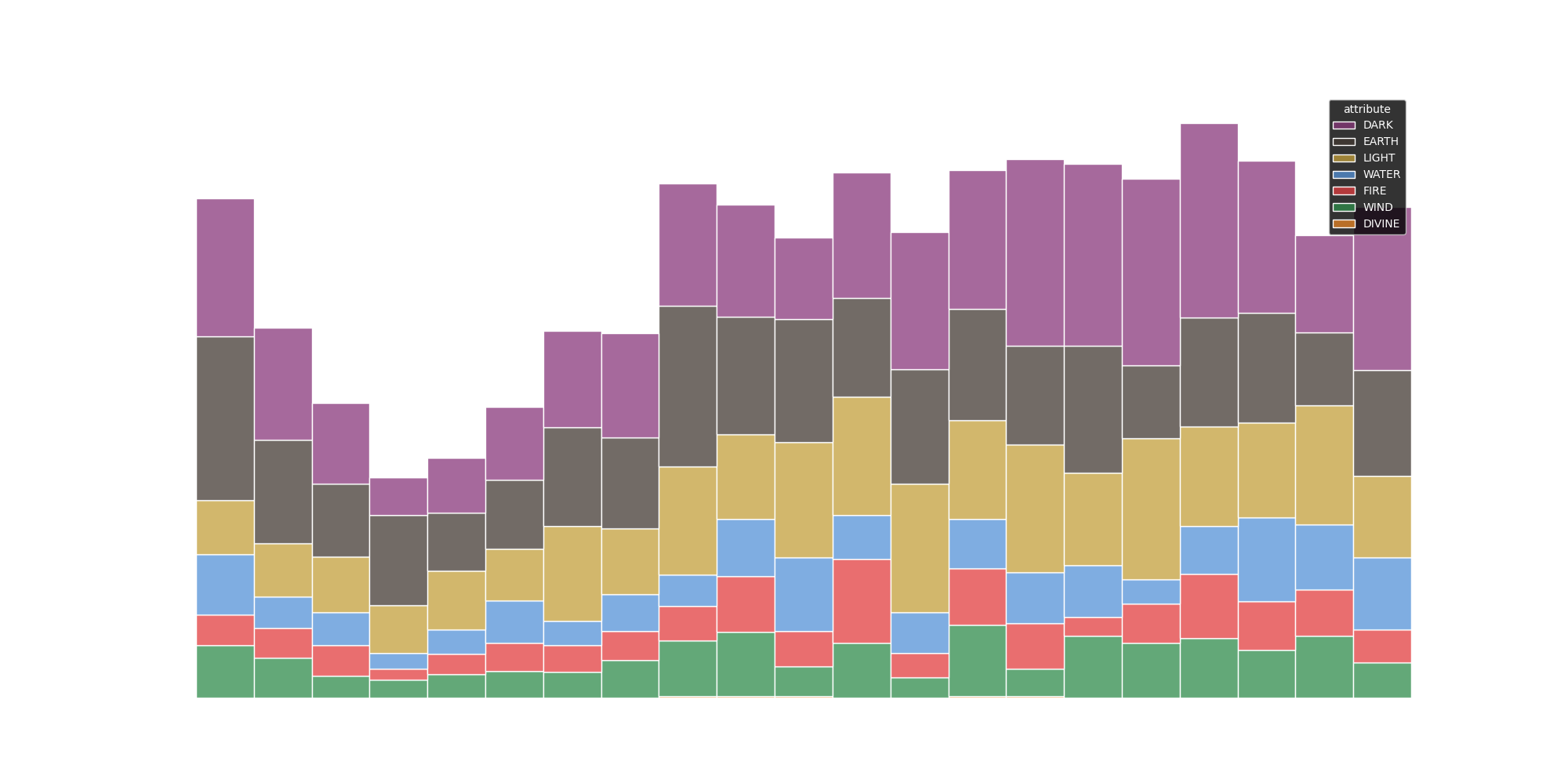 Number of cards by attribute
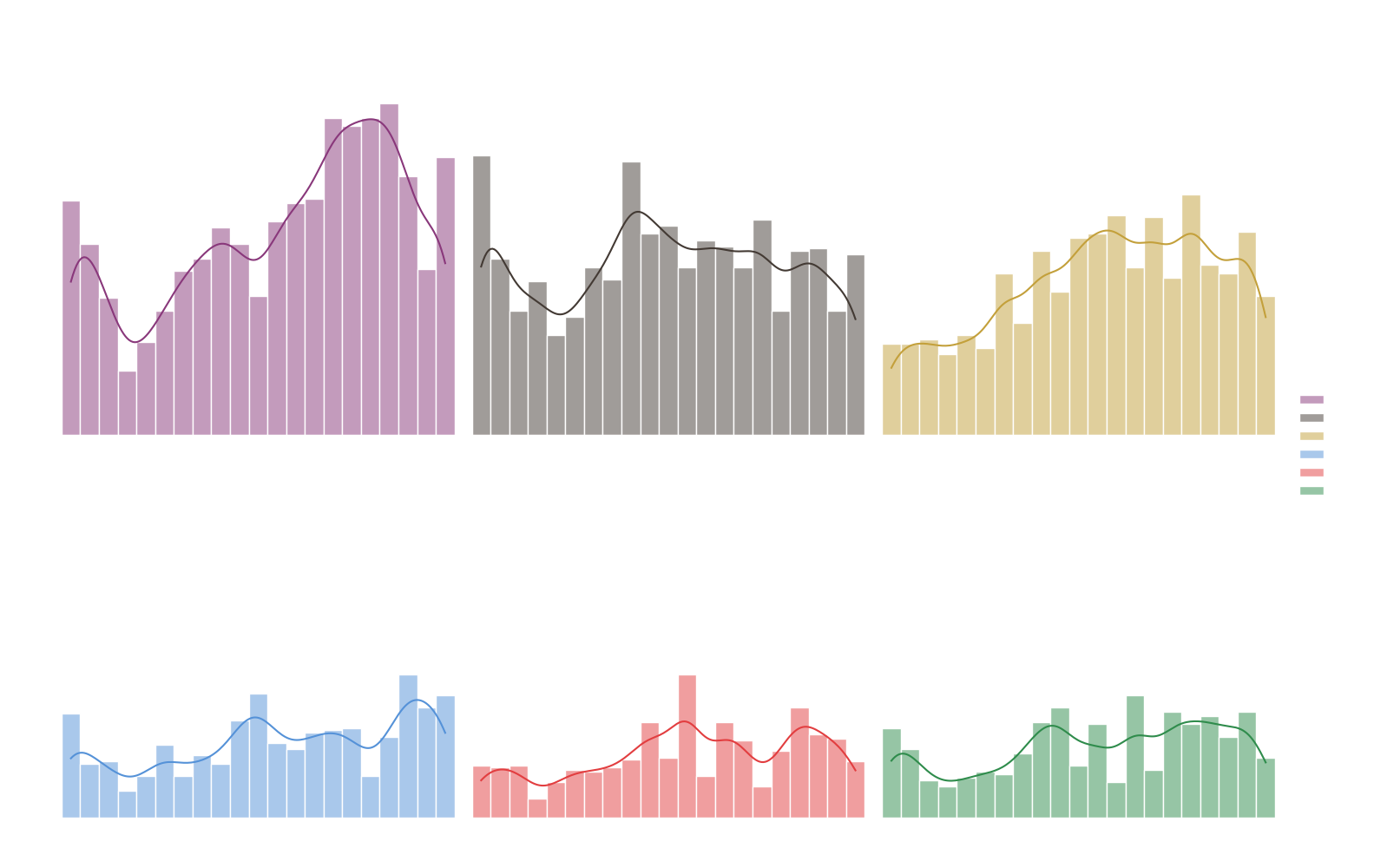
Although the overview is nice, comparing attributes in different years is still a bit hard. Apart from the bars representing the wind attribute (green), all the others start/end at a different height depending on the year. To solve that I opted for a new visualization making use of Seaborn’s FacetGrid.

Conclusion
Working with a YGO dataset was really interesting. I had some domain knowledge, and that made understanding the available information and how I should use it significantly easier. I also had the chance to practice my data visualization skills by creating some cool plots, using the techniques I found most suitable to answer the questions at hand.